Tutorial 4: Xenium (Hepatocellular Carcinoma)
This tutorial demonstrates how to:
Generate ligand-target neighborhood scores using Renoir for single-cell spatial data (Xenium)
Perform downstream spatial analysis using SpatialData, Scanpy, and Renoir
The workflow covers:
Ligand-target score computation for Xenium single-cell data
Communication domain discovery
Pathway activity scoring
Spatial visualization of ligand-target activity via SpatialData cell segmentation masks
Ligand ranking analysis
Cell type and Leiden cluster spatial plots
Dataset: Xenium HCC tumor sample
📥 Download processed data: The preprocessed input files required for this tutorial can be downloaded from:
https://zenodo.org/records/20078137After downloading, extract the archive and set the paths in Section 0 below.
0. Setup
[1]:
import Renoir
import scanpy as sc
import squidpy as sq
import spatialdata as sd
import spatialdata_plot
from spatialdata_io import xenium
import pandas as pd
import numpy as np
import pickle as pkl
import seaborn as sns
import matplotlib as mpl
import matplotlib.pyplot as plt
from matplotlib.patches import Patch
import distinctipy

mpl.rcParams['figure.dpi'] = 150
plt.rcParams['savefig.dpi'] = 300
plt.rcParams['figure.figsize'] = [8, 8]
/home/nr57/.conda/envs/genomics/lib/python3.11/site-packages/dask/dataframe/__init__.py:31: FutureWarning: The legacy Dask DataFrame implementation is deprecated and will be removed in a future version. Set the configuration option `dataframe.query-planning` to `True` or None to enable the new Dask Dataframe implementation and silence this warning.
  warnings.warn(
0.1 Set data paths
Update these paths to point to your downloaded data.
[ ]:
# ── Update these paths after downloading the data ──────────────────────────
SAMPLE          = 'Xenium'
DATA_ROOT       = '/path/to/Xenium/'          # <-- change this

# Input files (provided in the download)
SC_PATH         = f'{DATA_ROOT}/{SAMPLE}/filtered_sample_annotated.h5ad'
ST_PATH         = f'{DATA_ROOT}/{SAMPLE}/filtered_sample_annotated.h5ad'   # Xenium cell-level h5ad
CELLTYPE_PROP   = f'{DATA_ROOT}/{SAMPLE}/celltype_onehot.csv'
EXPINS_PATH     = f'{DATA_ROOT}/{SAMPLE}/mRNA_subset.pkl'
XENIUM_RAW_PATH = f'{DATA_ROOT}/raw/{SAMPLE}'         # raw Xenium output folder

# Reference files (provided in the download)
LT_PAIRS_PATH   = f'{DATA_ROOT}/top_100_target_opt_both_ordered.csv'
LR_PAIRS_PATH   = f'{DATA_ROOT}/All_human_lrpairs.csv'
LT_REG_POT_PATH = f'{DATA_ROOT}/top_500_target_opt_both_scores.pkl'
MSIG_PATH       = f'{DATA_ROOT}/msig_human_WP_H_KEGG.csv'

# Output paths
OUTPUT_DIR      = f'{DATA_ROOT}/{SAMPLE}'
SCORES_H5AD     = f'{OUTPUT_DIR}/{SAMPLE}_neighborhood_scores.h5ad'
# ──────────────────────────────────────────────────────────────────────────

import os
os.makedirs(OUTPUT_DIR, exist_ok=True)
print("Paths configured.")
Paths configured.
1. Generate Ligand-Target Neighborhood Scores with Renoir
For Xenium data, each cell is treated as an individual observation (single_cell=True). Renoir computes a ligand-target neighborhood score per cell by integrating cell-type identity, local neighborhood composition, and curated ligand-target regulatory potential.
[5]:
# Compute neighborhood scores
# For Xenium, single_cell=True and radius defines the search radius in µm
neighborhood_scores = Renoir.compute_neighborhood_scores(
    SC_path                   = SC_PATH,
    ST_path                   = ST_PATH,
    pairs_path                = LT_PAIRS_PATH,
    ligand_receptor_path      = LR_PAIRS_PATH,
    celltype_proportions_path = CELLTYPE_PROP,
    expins_path               = None,
    single_cell               = True,   # Xenium is single-cell resolution
    radius                    = 30,     # search radius in µm
)

neighborhood_scores.write_h5ad(SCORES_H5AD)
print(f"Scores saved to: {SCORES_H5AD}")
print(neighborhood_scores)
Loading datasets/celltypes
Loading expins
Fetching ligand/target pairs
157 ligand targets present
62 ligand target pairs present
100%|██████████| 157/157 [00:03<00:00, 40.35it/s]
Computing graph
Computing neighborhood scores
/home/nr57/.conda/envs/genomics/lib/python3.11/site-packages/Renoir/renoir.py:469: RuntimeWarning: invalid value encountered in divide
  PEM = np.log10(expins/E)
/home/nr57/.conda/envs/genomics/lib/python3.11/site-packages/Renoir/renoir.py:469: RuntimeWarning: divide by zero encountered in log10
  PEM = np.log10(expins/E)
Creating adata
Scores saved to: /shared/nr57/Renoir_data/Xenium//Tumor1/Tumor1_neighborhood_scores.h5ad
AnnData object with n_obs × n_vars = 139724 × 1010
    obs: 'cell_id', 'x_centroid', 'y_centroid', 'transcript_counts', 'control_probe_counts', 'genomic_control_counts', 'control_codeword_counts', 'unassigned_codeword_counts', 'deprecated_codeword_counts', 'total_counts', 'cell_area', 'nucleus_area', 'nucleus_count', 'segmentation_method', 'n_genes_by_counts', 'log1p_n_genes_by_counts', 'log1p_total_counts', 'pct_counts_in_top_10_genes', 'pct_counts_in_top_20_genes', 'pct_counts_in_top_50_genes', 'pct_counts_in_top_150_genes', 'n_counts', 'n_genes', 'keep', 'array_row', 'array_col', 'celltype', 'endothelial_level2', 'fibroblast_level2', 'myeloid_level2'
    var: 'gene_ids'
    uns: 'log1p', 'rank_genes_groups'
    obsm: 'spatial'
1.1 Reload pre-computed scores (skip if running from scratch)
[9]:
neighborhood_scores = sc.read_h5ad(SCORES_H5AD)
print(neighborhood_scores)
AnnData object with n_obs × n_vars = 139724 × 1010
    obs: 'cell_id', 'x_centroid', 'y_centroid', 'transcript_counts', 'control_probe_counts', 'genomic_control_counts', 'control_codeword_counts', 'unassigned_codeword_counts', 'deprecated_codeword_counts', 'total_counts', 'cell_area', 'nucleus_area', 'nucleus_count', 'segmentation_method', 'n_genes_by_counts', 'log1p_n_genes_by_counts', 'log1p_total_counts', 'pct_counts_in_top_10_genes', 'pct_counts_in_top_20_genes', 'pct_counts_in_top_50_genes', 'pct_counts_in_top_150_genes', 'n_counts', 'n_genes', 'keep', 'array_row', 'array_col', 'celltype', 'endothelial_level2', 'fibroblast_level2', 'myeloid_level2'
    var: 'gene_ids'
    uns: 'log1p', 'rank_genes_groups'
    obsm: 'spatial'
2. Pathway Clusters and Communication Domain Discovery
2.1 Build Pathway-Based Ligand-Target Clusters
[10]:
# Load MSigDB pathways
msig = Renoir.get_msig('custom', path=MSIG_PATH)

# Group ligand-target pairs into pathway clusters
pathways = Renoir.create_cluster(
    neighborhood_scores,
    msig,
    method         = None,
    restrict_to_KHW = True,
    pathway_thresh  = 20
)

print(f"Generated {len(pathways)} pathway clusters.")
print(list(pathways.keys())[:10], "...")
Generated 25 pathway clusters.
['HALLMARK_ALLOGRAFT_REJECTION', 'HALLMARK_EPITHELIAL_MESENCHYMAL_TRANSITION', 'HALLMARK_INFLAMMATORY_RESPONSE', 'HALLMARK_TNFA_SIGNALING_VIA_NFKB', 'KEGG_CHEMOKINE_SIGNALING_PATHWAY', 'KEGG_CYTOKINE_CYTOKINE_RECEPTOR_INTERACTION', 'KEGG_FOCAL_ADHESION', 'KEGG_PATHWAYS_IN_CANCER', 'WP_ALLOGRAFT_REJECTION', 'WP_BURN_WOUND_HEALING'] ...
2.2 Compute Communication Domains
[12]:
neighbscore_copy, pcs = Renoir.downstream_analysis(
    neighborhood_scores,
    ltpair_clusters = pathways,
    resolution      = 0.05,
    n_markers       = 20,
    n_top           = 20,
    pdf_path        = None,
    return_cluster  = True,
    return_pcs      = True,
)

# Transfer domain labels back to neighborhood_scores
neighborhood_scores.obs['leiden'] = neighbscore_copy.obs['leiden']
neighborhood_scores.uns           = neighbscore_copy.uns

print("Domains found:", neighborhood_scores.obs['leiden'].unique().tolist())
/home/nr57/.conda/envs/genomics/lib/python3.11/site-packages/scipy/sparse/_index.py:145: SparseEfficiencyWarning: Changing the sparsity structure of a csr_matrix is expensive. lil_matrix is more efficient.
  self._set_arrayXarray(i, j, x)
/home/nr57/.conda/envs/genomics/lib/python3.11/site-packages/scipy/sparse/_index.py:145: SparseEfficiencyWarning: Changing the sparsity structure of a csr_matrix is expensive. lil_matrix is more efficient.
  self._set_arrayXarray(i, j, x)
Domains found: ['0', '1', '3', '5', '8', '2', '4', '7', '6', '12', '9', '10', '11', '13']
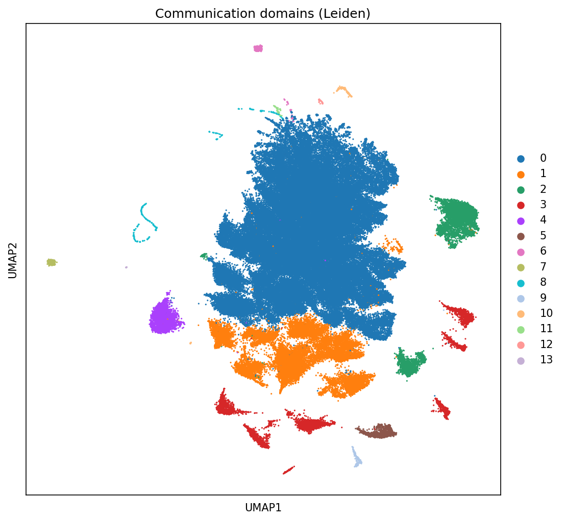
2.3 UMAP of Communication Domains
[13]:
sc.pl.umap(neighbscore_copy, color='leiden', size=9, title='Communication domains (Leiden)')
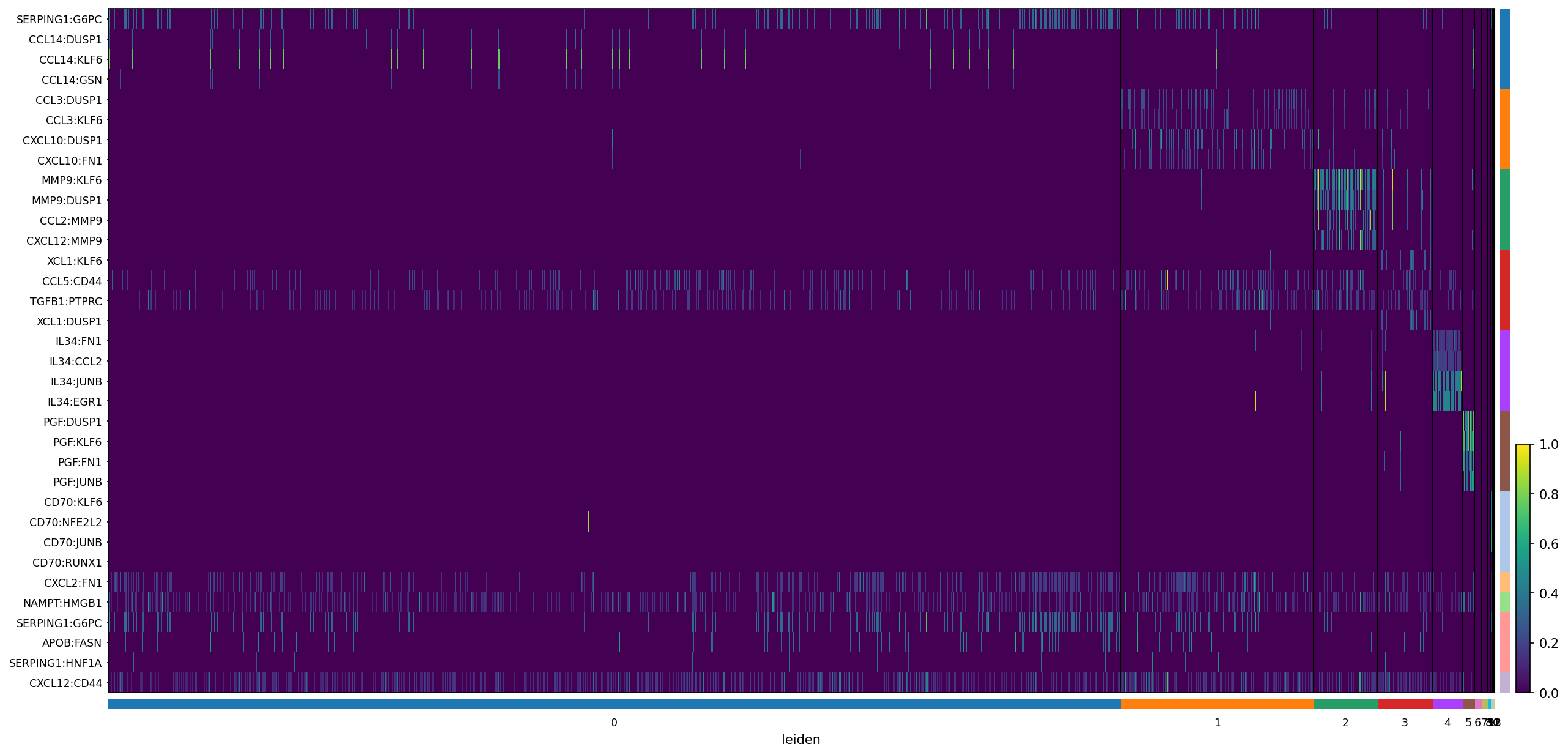
3. Differential Expression Across Communication Domains
[15]:
sc.tl.rank_genes_groups(neighborhood_scores, groupby='leiden', method='wilcoxon')

sc.pl.rank_genes_groups_heatmap(
    neighborhood_scores,
    n_genes           = 4,
    groupby           = 'leiden',
    show_gene_labels  = True,
    min_logfoldchange = 0.5,
    dendrogram        = False,
    swap_axes         = True,
    standard_scale    = 'var',
    cmap              = 'viridis',
    figsize           = (20, 10),
)
WARNING: No genes found for group 6
WARNING: No genes found for group 7
WARNING: No genes found for group 8
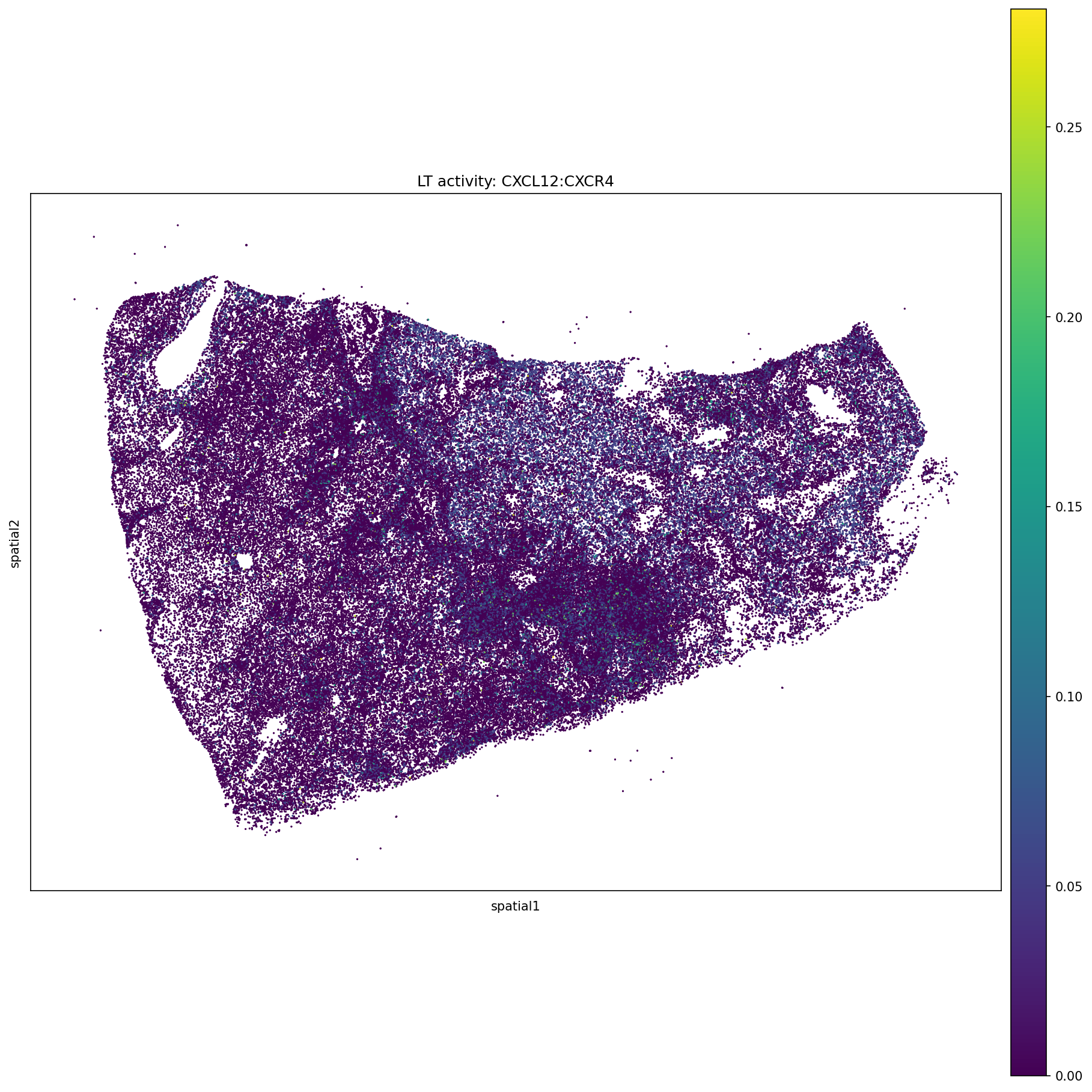
4. Spatial Plots via Squidpy (quick overview)
We use Squidpy for a fast scatter plot overview before moving to the full SpatialData pipeline.
[16]:
# Example ligand-target pair — update to a pair present in your data
EXAMPLE_PAIR = 'CXCL12:CXCR4'

sq.pl.spatial_scatter(
    neighborhood_scores,
    library_id = 'spatial',
    shape      = None,
    color      = [EXAMPLE_PAIR],
    figsize    = (12, 12),
    title      = f'LT activity: {EXAMPLE_PAIR}',
)
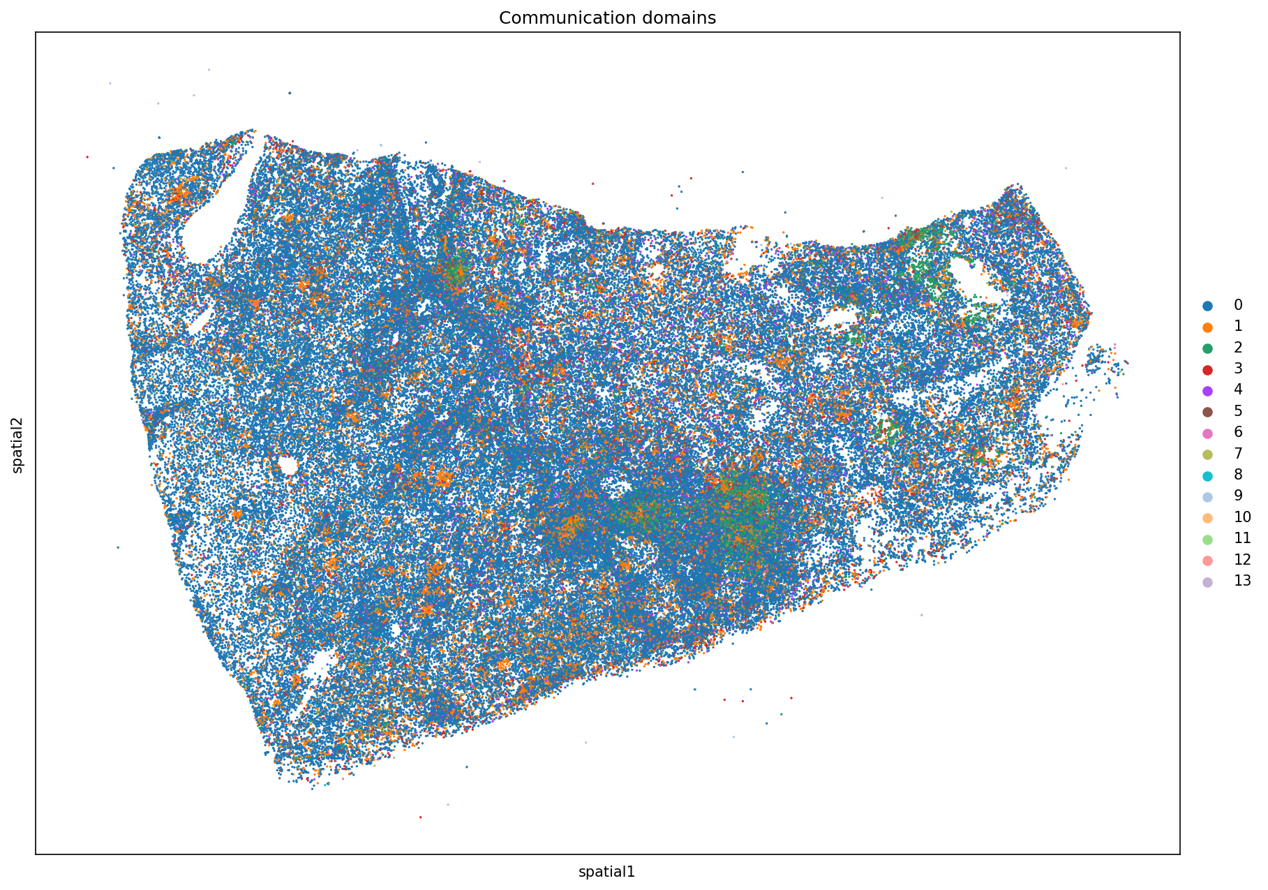
[17]:
sq.pl.spatial_scatter(
    neighborhood_scores,
    library_id = 'spatial',
    shape      = None,
    color      = ['leiden'],
    figsize    = (12, 12),
    title      = 'Communication domains',
)
/home/nr57/.conda/envs/genomics/lib/python3.11/site-packages/squidpy/pl/_spatial_utils.py:956: UserWarning: No data for colormapping provided via 'c'. Parameters 'cmap', 'norm' will be ignored
  _cax = scatter(
5. SpatialData — Cell Segmentation Mask Plots
5.1 Build the SpatialData object from raw Xenium output
[21]:
# Build SpatialData from raw Xenium output directory
sdata = xenium(XENIUM_RAW_PATH)
print(sdata)
/tmp/ipykernel_82268/1266032761.py:2: DeprecationWarning: The default value of `cells_as_circles` will change to `False` in the next release. Please pass `True` explicitly to maintain the current behavior.
  sdata = xenium(XENIUM_RAW_PATH)
INFO     reading /shared/nr57/Renoir_data/Xenium/raw/M293/cell_feature_matrix.h5
SpatialData object
├── Images
│     └── 'morphology_focus': DataTree[cyx] (4, 27280, 39815), (4, 13640, 19907), (4, 6820, 9953), (4, 3410, 4976), (4, 1705, 2488)
├── Labels
│     ├── 'cell_labels': DataTree[yx] (27280, 39815), (13640, 19907), (6820, 9953), (3410, 4976), (1705, 2488)
│     └── 'nucleus_labels': DataTree[yx] (27280, 39815), (13640, 19907), (6820, 9953), (3410, 4976), (1705, 2488)
├── Points
│     └── 'transcripts': DataFrame with shape: (<Delayed>, 13) (3D points)
├── Shapes
│     ├── 'cell_boundaries': GeoDataFrame shape: (155148, 1) (2D shapes)
│     ├── 'cell_circles': GeoDataFrame shape: (155148, 2) (2D shapes)
│     └── 'nucleus_boundaries': GeoDataFrame shape: (149720, 1) (2D shapes)
└── Tables
      └── 'table': AnnData (155148, 319)
with coordinate systems:
    ▸ 'global', with elements:
        morphology_focus (Images), cell_labels (Labels), nucleus_labels (Labels), transcripts (Points), cell_boundaries (Shapes), cell_circles (Shapes), nucleus_boundaries (Shapes)
5.2 Align SpatialData to the filtered neighborhood scores
Filter the SpatialData table and cell boundary shapes to only cells that passed QC and are present in neighborhood_scores.
[22]:
adata = sdata.table

# Keep only cells present in neighborhood_scores
filtered_adata = adata[adata.obs['cell_id'].isin(neighborhood_scores.obs['cell_id'])].copy()
filtered_adata.obs = filtered_adata.obs.set_index('cell_id')
filtered_adata.obs['cell_id'] = filtered_adata.obs.index

# Filter matching cell boundary shapes
filtered_shapes = sdata.shapes['cell_boundaries'].loc[
    sdata.shapes['cell_boundaries'].index.isin(filtered_adata.obs.index)
].copy()

print(f"Cells retained: {len(filtered_adata)}")
Cells retained: 139724
/tmp/ipykernel_82268/886675138.py:1: DeprecationWarning: Table accessor will be deprecated with SpatialData version 0.1, use sdata.tables instead.
  adata = sdata.table
/home/nr57/.conda/envs/genomics/lib/python3.11/site-packages/anndata/_core/anndata.py:183: ImplicitModificationWarning: Transforming to str index.
  warnings.warn("Transforming to str index.", ImplicitModificationWarning)
[23]:
# Transfer cell type and Leiden domain labels
for col in ['celltype', 'leiden']:
    filtered_adata.obs[col]  = neighborhood_scores.obs[col].reindex(filtered_adata.obs.index)
    filtered_shapes[col]     = filtered_adata.obs[col]

# Build the filtered SpatialData object
sdata_filtered = sd.SpatialData(
    tables = {'table': filtered_adata},
    shapes = {'cell_boundaries': filtered_shapes},
    images = sdata.images,
    labels = sdata.labels,
    points = sdata.points,
)

print(sdata_filtered)
SpatialData object
├── Images
│     └── 'morphology_focus': DataTree[cyx] (4, 27280, 39815), (4, 13640, 19907), (4, 6820, 9953), (4, 3410, 4976), (4, 1705, 2488)
├── Labels
│     ├── 'cell_labels': DataTree[yx] (27280, 39815), (13640, 19907), (6820, 9953), (3410, 4976), (1705, 2488)
│     └── 'nucleus_labels': DataTree[yx] (27280, 39815), (13640, 19907), (6820, 9953), (3410, 4976), (1705, 2488)
├── Points
│     └── 'transcripts': DataFrame with shape: (<Delayed>, 13) (3D points)
├── Shapes
│     └── 'cell_boundaries': GeoDataFrame shape: (139724, 3) (2D shapes)
└── Tables
      └── 'table': AnnData (139724, 319)
with coordinate systems:
    ▸ 'global', with elements:
        morphology_focus (Images), cell_labels (Labels), nucleus_labels (Labels), transcripts (Points), cell_boundaries (Shapes)
/home/nr57/.conda/envs/genomics/lib/python3.11/site-packages/spatialdata/_core/spatialdata.py:184: UserWarning: The table is annotating 'cell_circles', which is not present in the SpatialData object.
  self.validate_table_in_spatialdata(v)
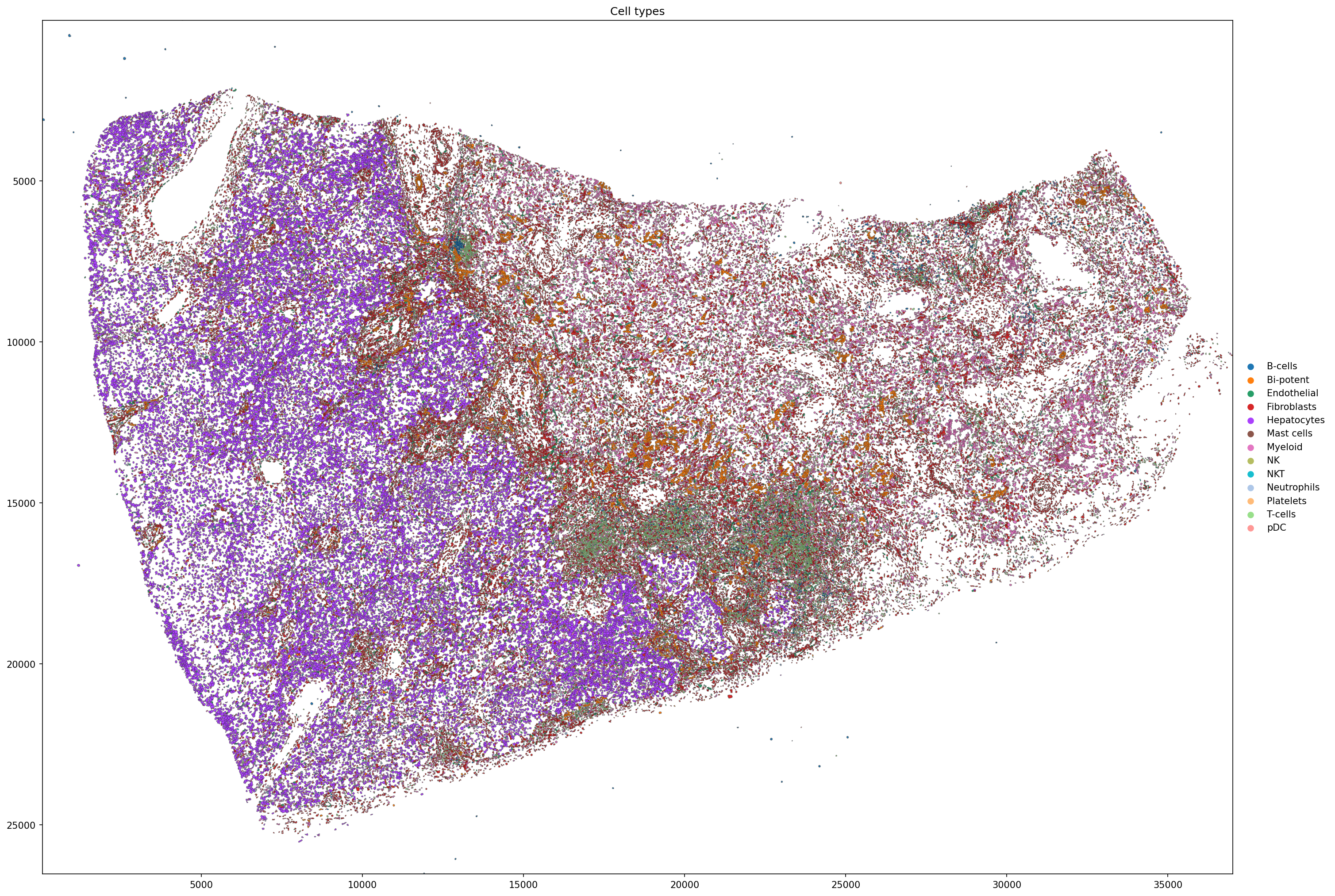
5.3 Spatial map of cell types
[24]:
sdata_filtered.pl.render_shapes(
    element         = 'cell_boundaries',
    color           = 'celltype',
    color_continuous = False,
    outline_alpha   = 0.5,
    outline_width   = 0.5,
).pl.show(
    coordinate_systems = 'global',
    figsize            = (20, 20),
    title              = 'Cell types',
)
INFO     Using 'datashader' backend with 'None' as reduction method to speed up plotting. Depending on the
         reduction method, the value range of the plot might change. Set method to 'matplotlib' to disable this
         behaviour.
/home/nr57/.conda/envs/genomics/lib/python3.11/site-packages/spatialdata/_core/spatialdata.py:184: UserWarning: The table is annotating 'cell_circles', which is not present in the SpatialData object.
  self.validate_table_in_spatialdata(v)
/home/nr57/.conda/envs/genomics/lib/python3.11/site-packages/spatialdata/_core/spatialdata.py:184: UserWarning: The table is annotating 'cell_circles', which is not present in the SpatialData object.
  self.validate_table_in_spatialdata(v)
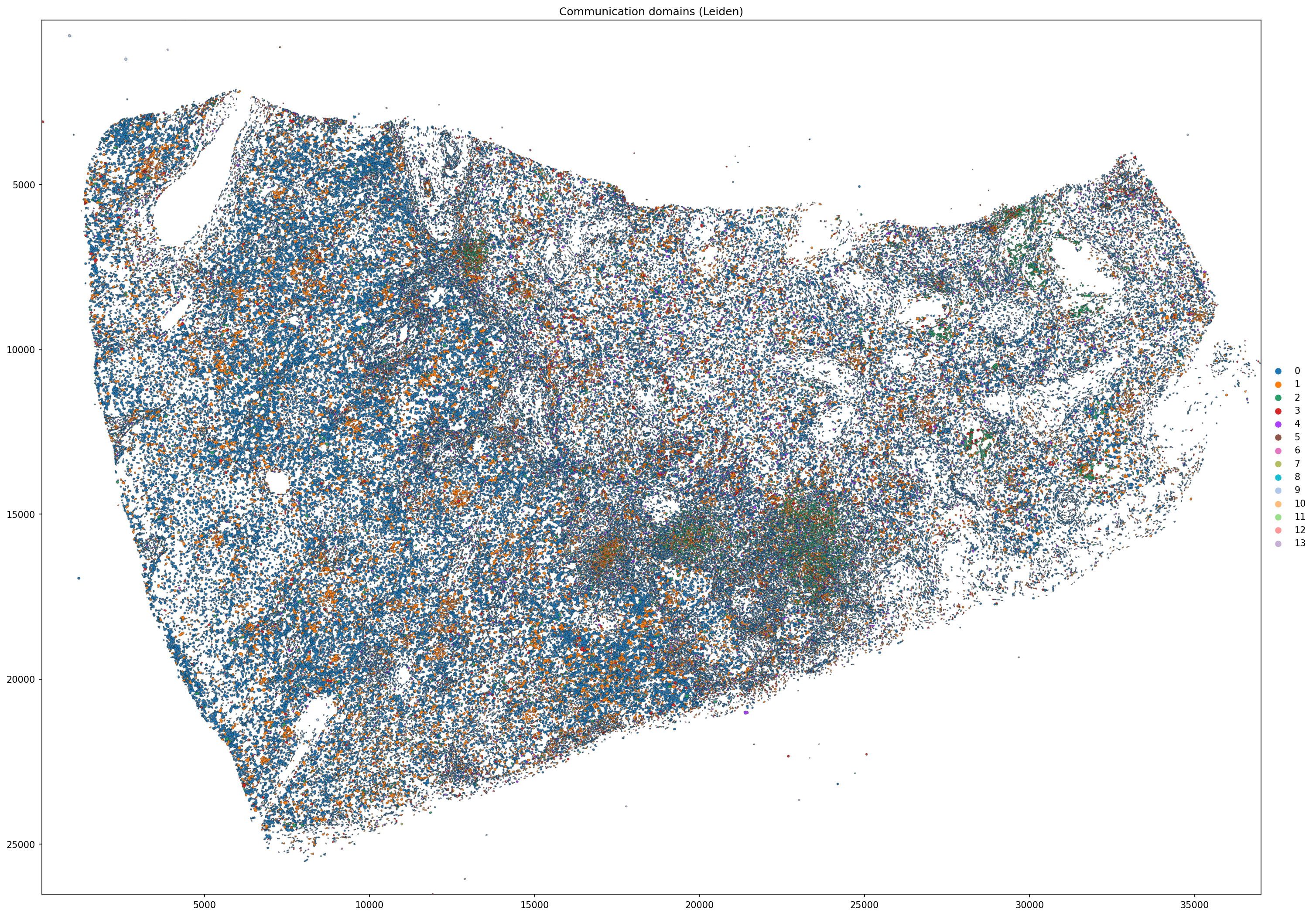
5.4 Spatial map of Leiden communication domains
[25]:
sdata_filtered.pl.render_shapes(
    element         = 'cell_boundaries',
    color           = 'leiden',
    color_continuous = False,
    outline_alpha   = 0.5,
    outline_width   = 0.5,
).pl.show(
    coordinate_systems = 'global',
    figsize            = (20, 20),
    title              = 'Communication domains (Leiden)',
)
INFO     Using 'datashader' backend with 'None' as reduction method to speed up plotting. Depending on the
         reduction method, the value range of the plot might change. Set method to 'matplotlib' to disable this
         behaviour.
/home/nr57/.conda/envs/genomics/lib/python3.11/site-packages/spatialdata/_core/spatialdata.py:184: UserWarning: The table is annotating 'cell_circles', which is not present in the SpatialData object.
  self.validate_table_in_spatialdata(v)
/home/nr57/.conda/envs/genomics/lib/python3.11/site-packages/spatialdata/_core/spatialdata.py:184: UserWarning: The table is annotating 'cell_circles', which is not present in the SpatialData object.
  self.validate_table_in_spatialdata(v)
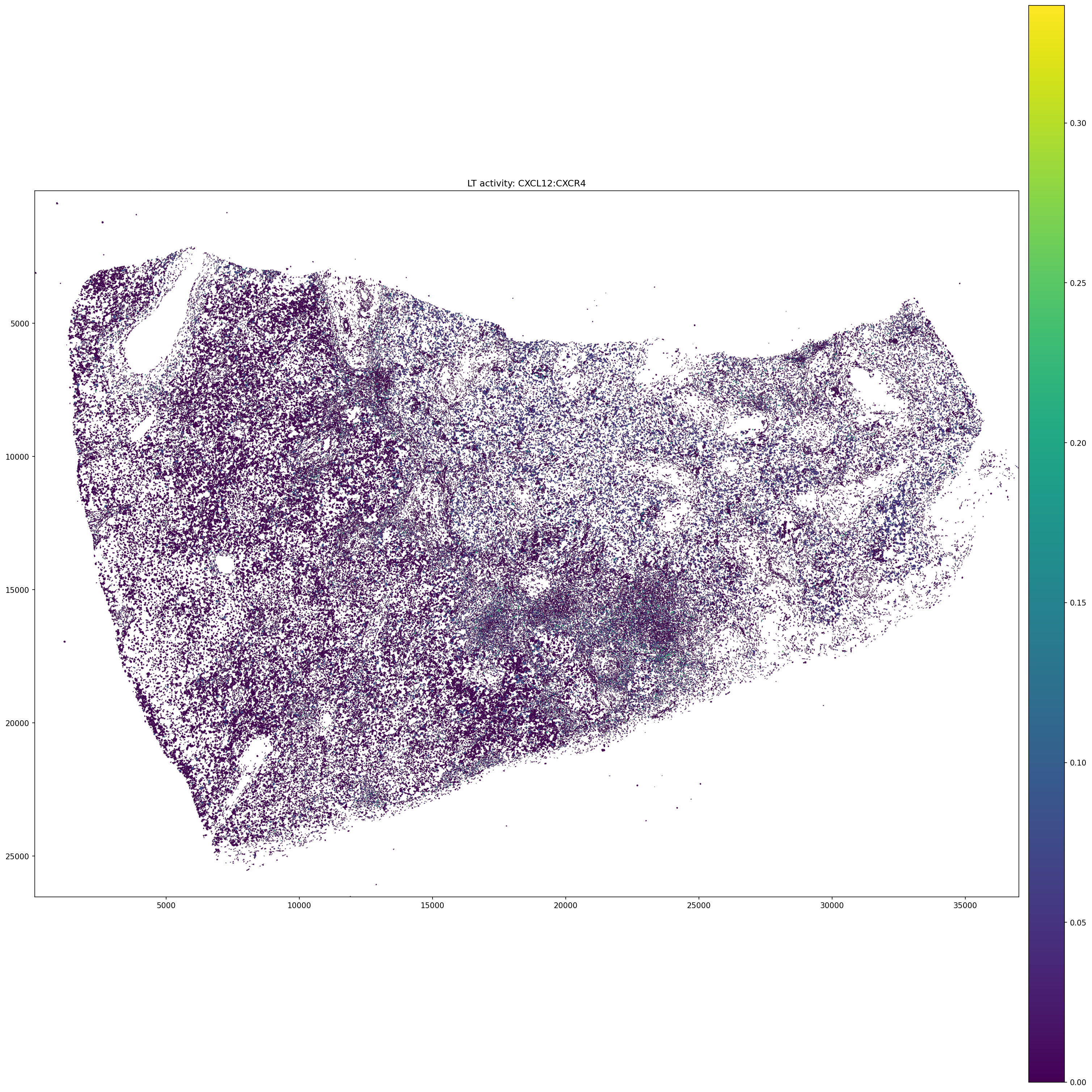
5.5 Spatial map of example ligand-target activity
[26]:
# Inject LT activity score into shapes for spatial plotting
fixed_pair = EXAMPLE_PAIR.replace(':', '_')
lt_scores  = neighborhood_scores[:, EXAMPLE_PAIR].X

lt_scores_df = pd.DataFrame(
    lt_scores,
    index   = neighborhood_scores.obs.index,
    columns = [fixed_pair],
)

sdata_filtered.tables['table'].obs = sdata_filtered.tables['table'].obs.merge(
    lt_scores_df, left_index=True, right_index=True, how='left'
)
sdata_filtered.shapes['cell_boundaries'][fixed_pair] = (
    sdata_filtered.tables['table'].obs[fixed_pair]
)

sdata_filtered.pl.render_shapes(
    element          = 'cell_boundaries',
    color            = fixed_pair,
    color_continuous = True,
    outline_alpha    = 0.3,
    outline_width    = 0.5,
).pl.show(
    coordinate_systems = 'global',
    figsize            = (20, 20),
    title              = f'LT activity: {EXAMPLE_PAIR}',
)
INFO     Using 'datashader' backend with 'None' as reduction method to speed up plotting. Depending on the
         reduction method, the value range of the plot might change. Set method to 'matplotlib' to disable this
         behaviour.
/home/nr57/.conda/envs/genomics/lib/python3.11/site-packages/spatialdata/_core/spatialdata.py:184: UserWarning: The table is annotating 'cell_circles', which is not present in the SpatialData object.
  self.validate_table_in_spatialdata(v)
/home/nr57/.conda/envs/genomics/lib/python3.11/site-packages/spatialdata/_core/spatialdata.py:184: UserWarning: The table is annotating 'cell_circles', which is not present in the SpatialData object.
  self.validate_table_in_spatialdata(v)
INFO Using the datashader reduction "mean". "max" will give an output very close to the matplotlib result.
5.6 Zoomed-in region of interest
Subset to a bounding box to inspect cell-level detail.
[ ]:
# Adjust coordinates to your region of interest
x_min, x_max = 3700, 4100
y_min, y_max = 3800, 4400
roi_mask = (
filtered_shapes.geometry.centroid.x.between(x_min, x_max) &
filtered_shapes.geometry.centroid.y.between(y_min, y_max)
)
filtered_adata.obs[EXAMPLE_PAIR.replace(':','_')] = neighborhood_scores.to_df()[EXAMPLE_PAIR].copy() #injecting neighborhood scores. To incorporate all neighborhood scores, see function register_table
shapes_roi = filtered_shapes[roi_mask]
adata_roi = filtered_adata[filtered_adata.obs.index.isin(shapes_roi.index)]
sdata_roi = sd.SpatialData(
tables = {'table': adata_roi},
shapes = {'cell_boundaries': shapes_roi},
images = sdata.images,
labels = sdata.labels,
points = sdata.points,
)
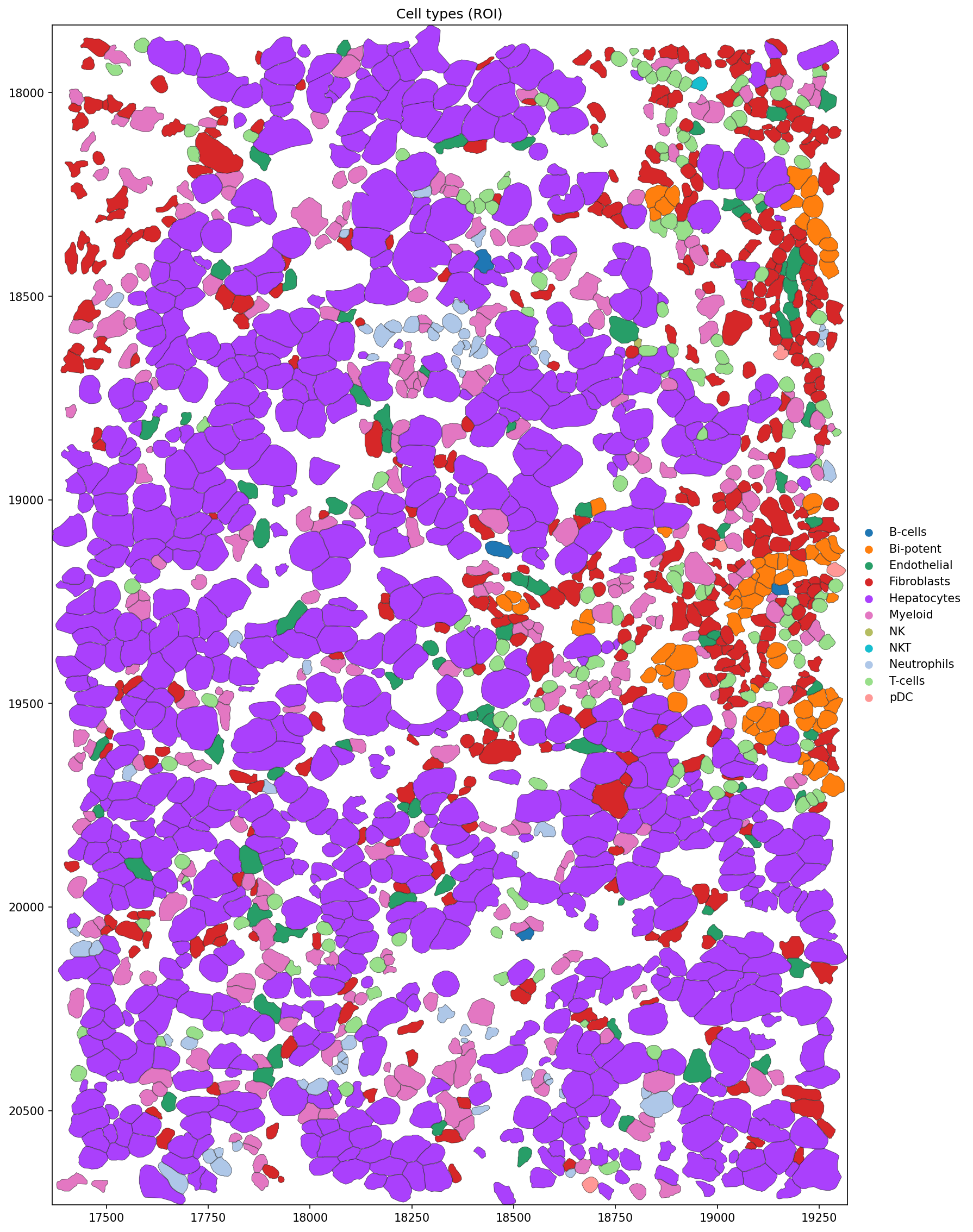
sdata_roi.pl.render_shapes(
element = 'cell_boundaries',
color = 'celltype',
color_continuous = False,
outline_alpha = 0.5,
outline_width = 0.5,
).pl.show(
coordinate_systems = 'global',
figsize = (15, 15),
title = 'Cell types (ROI)',
)
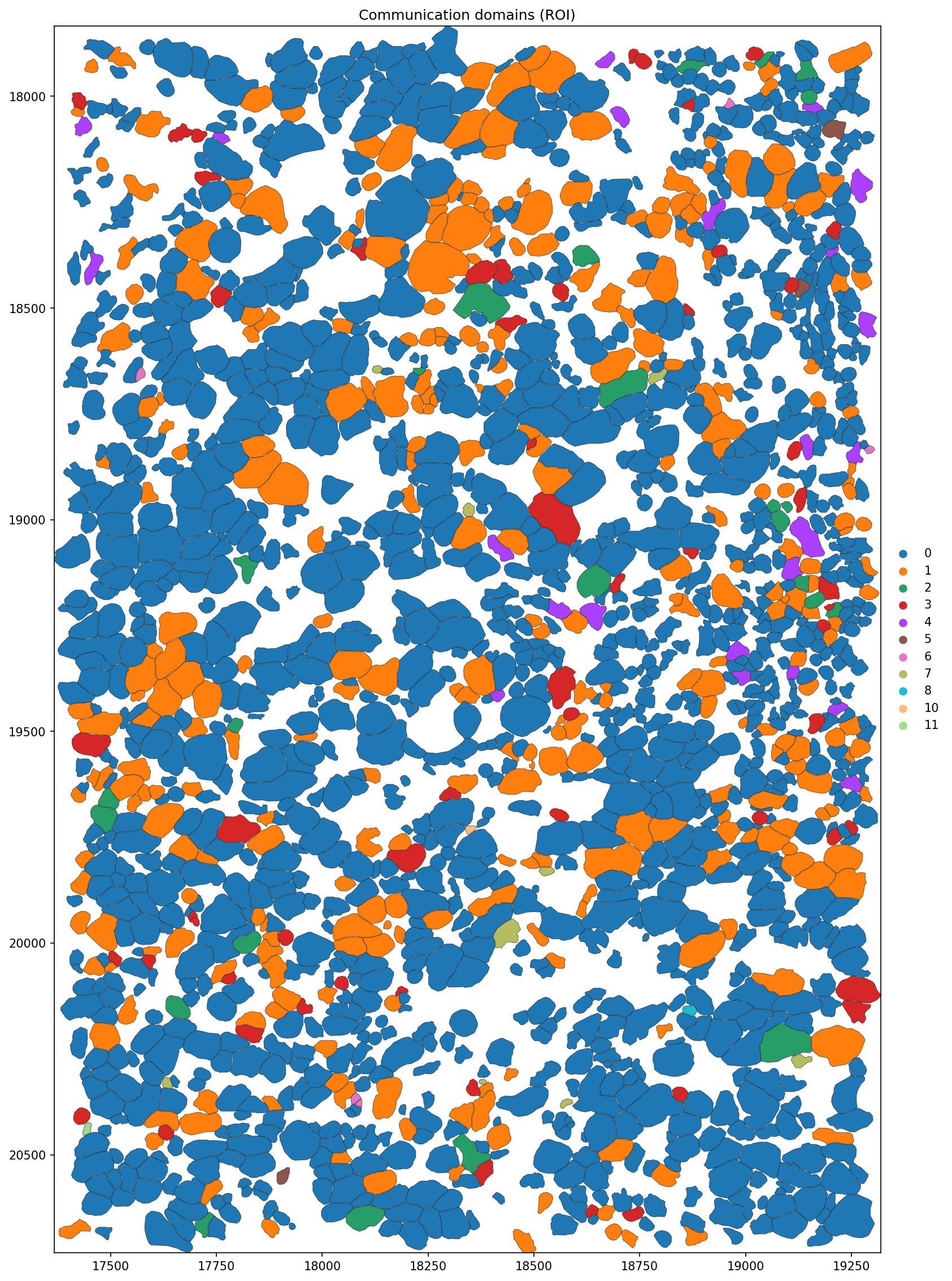
sdata_roi.pl.render_shapes(
element = 'cell_boundaries',
color = 'leiden',
color_continuous = False,
outline_alpha = 0.5,
outline_width = 0.5,
).pl.show(
coordinate_systems = 'global',
figsize = (15, 15),
title = 'Communication domains (ROI)',
)
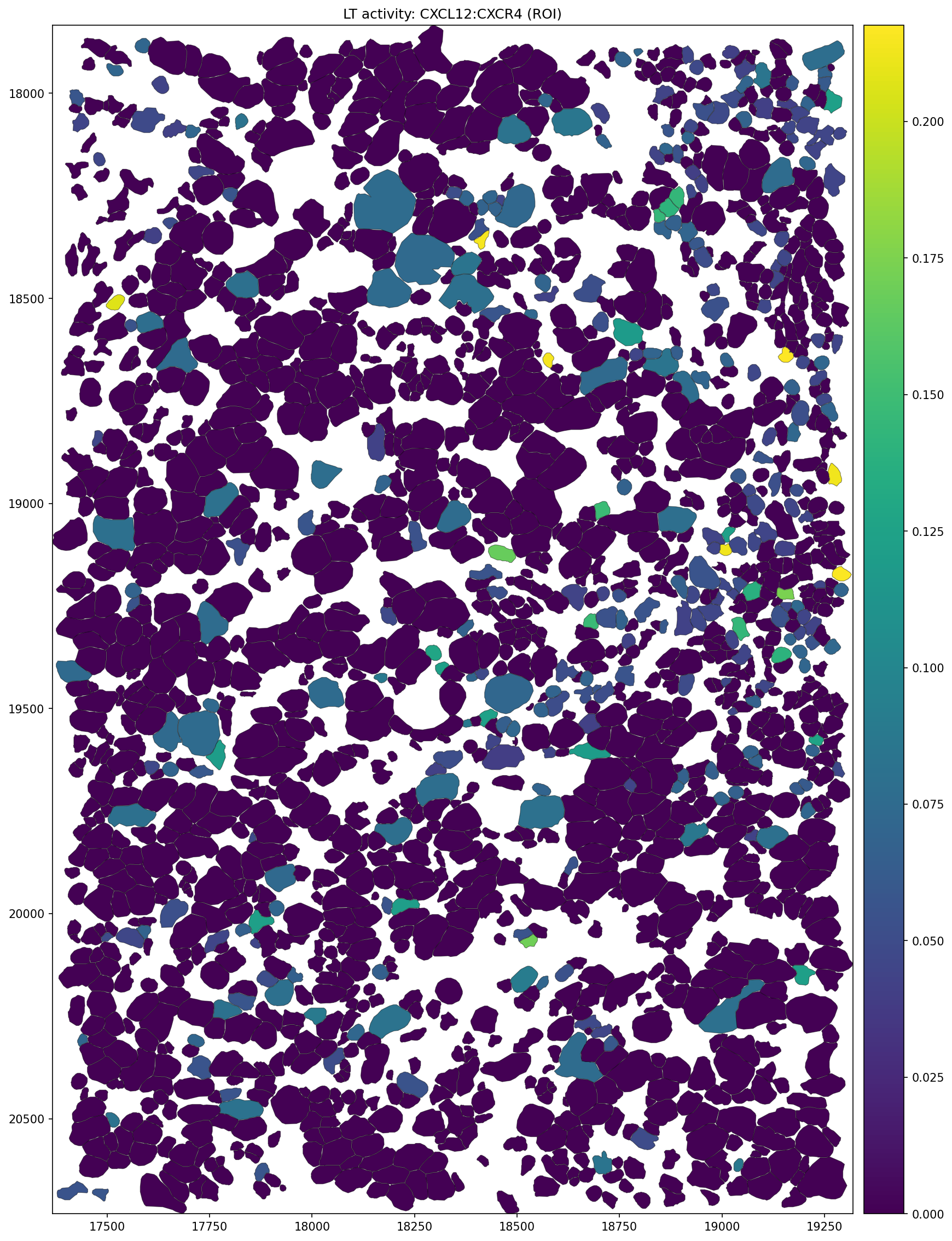
sdata_roi.pl.render_shapes(
element = 'cell_boundaries',
color = EXAMPLE_PAIR.replace(':','_'),
color_continuous = False,
outline_alpha = 0.5,
outline_width = 0.5,
).pl.show(
coordinate_systems = 'global',
figsize = (15, 15),
title = f'LT activity: {EXAMPLE_PAIR} (ROI)',
)
/home/nr57/.conda/envs/genomics/lib/python3.11/site-packages/spatialdata/_core/spatialdata.py:184: UserWarning: The table is annotating 'cell_circles', which is not present in the SpatialData object.
  self.validate_table_in_spatialdata(v)
/home/nr57/.conda/envs/genomics/lib/python3.11/site-packages/spatialdata/_core/spatialdata.py:184: UserWarning: The table is annotating 'cell_circles', which is not present in the SpatialData object.
  self.validate_table_in_spatialdata(v)
/home/nr57/.conda/envs/genomics/lib/python3.11/site-packages/spatialdata/_core/spatialdata.py:184: UserWarning: The table is annotating 'cell_circles', which is not present in the SpatialData object.
  self.validate_table_in_spatialdata(v)
/home/nr57/.conda/envs/genomics/lib/python3.11/site-packages/spatialdata/_core/spatialdata.py:184: UserWarning: The table is annotating 'cell_circles', which is not present in the SpatialData object.
  self.validate_table_in_spatialdata(v)
/home/nr57/.conda/envs/genomics/lib/python3.11/site-packages/spatialdata/_core/spatialdata.py:184: UserWarning: The table is annotating 'cell_circles', which is not present in the SpatialData object.
  self.validate_table_in_spatialdata(v)
/home/nr57/.conda/envs/genomics/lib/python3.11/site-packages/spatialdata/_core/spatialdata.py:184: UserWarning: The table is annotating 'cell_circles', which is not present in the SpatialData object.
  self.validate_table_in_spatialdata(v)
6. Pathway Activity in PC Space
The pcs object contains spot-level pathway activity scores derived from the LT-pair PC decomposition.
[35]:
print("Available pathway PCs:")
print(pcs.var_names.tolist())
Available pathway PCs:
['HALLMARK_ALLOGRAFT_REJECTION', 'HALLMARK_EPITHELIAL_MESENCHYMAL_TRANSITION', 'HALLMARK_INFLAMMATORY_RESPONSE', 'HALLMARK_TNFA_SIGNALING_VIA_NFKB', 'KEGG_CHEMOKINE_SIGNALING_PATHWAY', 'KEGG_CYTOKINE_CYTOKINE_RECEPTOR_INTERACTION', 'KEGG_FOCAL_ADHESION', 'KEGG_PATHWAYS_IN_CANCER', 'WP_ALLOGRAFT_REJECTION', 'WP_BURN_WOUND_HEALING', 'WP_EPITHELIAL_TO_MESENCHYMAL_TRANSITION_IN_COLORECTAL_CANCER', 'WP_FOCAL_ADHESION', 'WP_FOCAL_ADHESION_PI3KAKTMTORSIGNALING_PATHWAY', 'WP_IL18_SIGNALING_PATHWAY', 'WP_LUNG_FIBROSIS', 'WP_MALIGNANT_PLEURAL_MESOTHELIOMA', 'WP_NETWORK_MAP_OF_SARSCOV2_SIGNALING_PATHWAY', 'WP_NUCLEAR_RECEPTORS_METAPATHWAY', 'WP_OREXIN_RECEPTOR_PATHWAY', 'WP_OVERVIEW_OF_PROINFLAMMATORY_AND_PROFIBROTIC_MEDIATORS', 'WP_PI3KAKT_SIGNALING_PATHWAY', 'WP_PROSTAGLANDIN_SIGNALING', 'WP_SARSCOV2_INNATE_IMMUNITY_EVASION_AND_CELLSPECIFIC_IMMUNE_RESPONSE', 'WP_SPINAL_CORD_INJURY', 'WP_VEGFAVEGFR2_SIGNALING_PATHWAY']
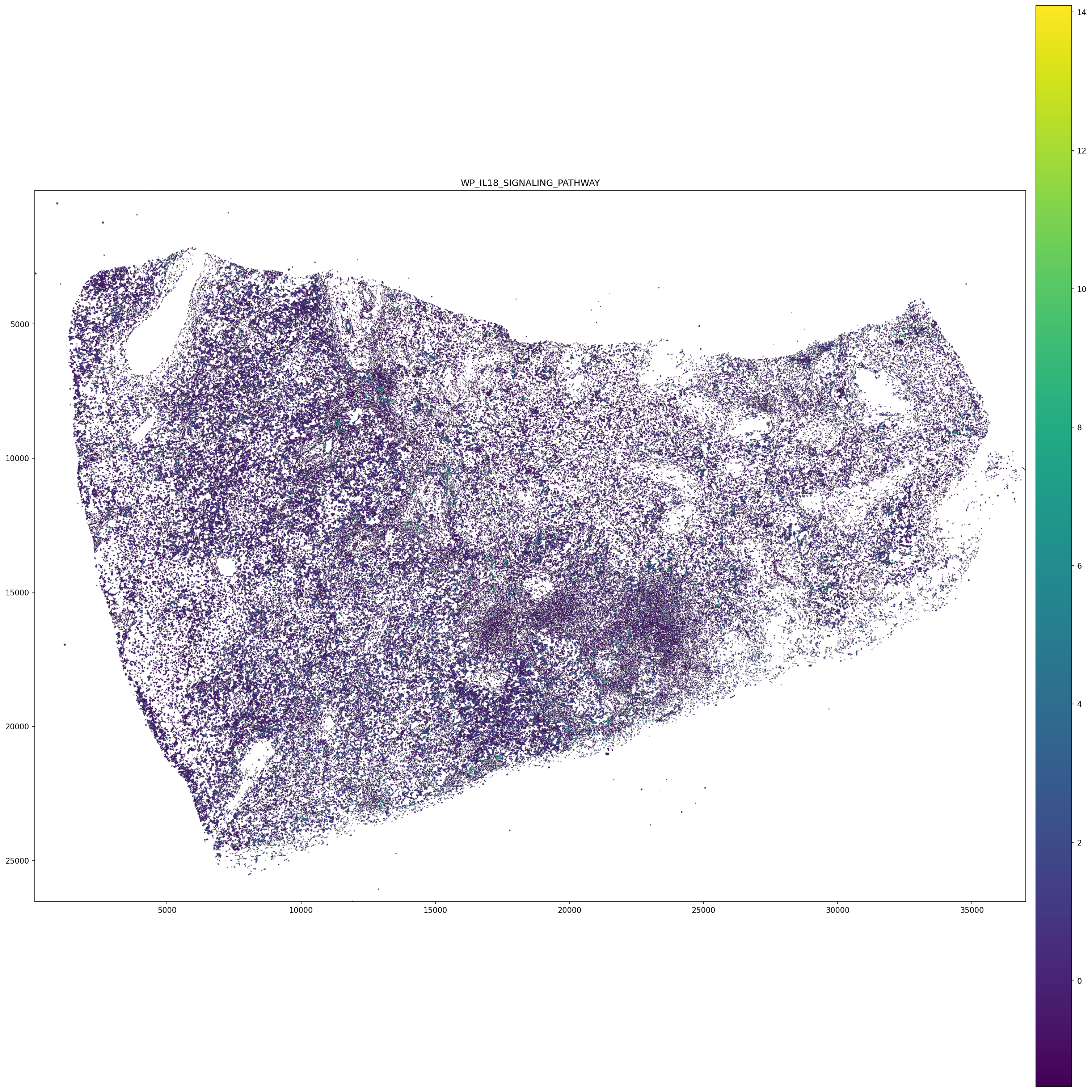
[36]:
# Visualize a pathway of interest spatially
# Replace with a pathway present in pcs.var_names
PATHWAY = 'WP_IL18_SIGNALING_PATHWAY'

if PATHWAY in pcs.var_names:
    pw_scores = pcs[:, PATHWAY].X
    pw_scores = pw_scores.toarray().ravel() if hasattr(pw_scores, 'toarray') else pw_scores.ravel()

    pw_df = pd.DataFrame(pw_scores, index=pcs.obs_names, columns=[PATHWAY])

    sdata_filtered.tables['table'].obs = sdata_filtered.tables['table'].obs.merge(
        pw_df, left_index=True, right_index=True, how='left'
    )
    sdata_filtered.shapes['cell_boundaries'][PATHWAY] = (
        sdata_filtered.tables['table'].obs[PATHWAY].fillna(0)
    )

    sdata_filtered.pl.render_shapes(
        element          = 'cell_boundaries',
        color            = PATHWAY,
        color_continuous = True,
        outline_alpha    = 0.3,
        outline_width    = 0.5,
    ).pl.show(
        coordinate_systems = 'global',
        figsize            = (20, 20),
        title              = PATHWAY,
    )
else:
    print(f"{PATHWAY} not found. Choose from: {pcs.var_names.tolist()}")
INFO     Using 'datashader' backend with 'None' as reduction method to speed up plotting. Depending on the
         reduction method, the value range of the plot might change. Set method to 'matplotlib' to disable this
         behaviour.
/home/nr57/.conda/envs/genomics/lib/python3.11/site-packages/spatialdata/_core/spatialdata.py:184: UserWarning: The table is annotating 'cell_circles', which is not present in the SpatialData object.
  self.validate_table_in_spatialdata(v)
/home/nr57/.conda/envs/genomics/lib/python3.11/site-packages/spatialdata/_core/spatialdata.py:184: UserWarning: The table is annotating 'cell_circles', which is not present in the SpatialData object.
  self.validate_table_in_spatialdata(v)
INFO Using the datashader reduction "mean". "max" will give an output very close to the matplotlib result.
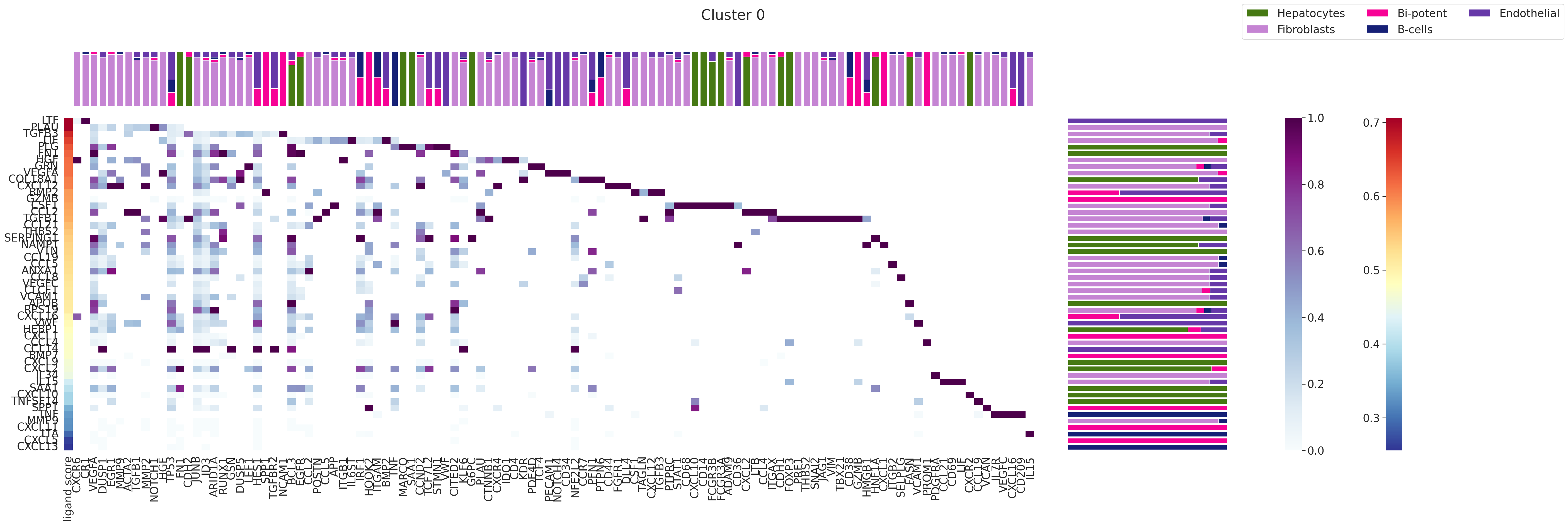
7. Ligand Ranking Analysis
Renoir.ligand_ranking ranks ligands within a selected communication domain by correlating their LT activity scores with known regulatory potential scores.
Inputs required:
Argument |
Description |
|---|---|
|
Renoir output AnnData (with |
|
Cell-type proportion AnnData (cells × cell types) |
|
Single-cell reference AnnData (with |
|
DataFrame of known L-R pairs ( |
|
Dict |
|
Leiden cluster label to analyse |
[38]:
# Load reference files
ligand_receptor_pairs              = pd.read_csv(LR_PAIRS_PATH)
ligand_target_regulatory_potential = pkl.load(open(LT_REG_POT_PATH, 'rb'))
SC = sc.read_h5ad(SC_PATH)

# Standardise the cell-type column name if needed
if 'cellType' in SC.obs.columns and 'celltype' not in SC.obs.columns:
    SC.obs['celltype'] = SC.obs['cellType']

# Build the cell-type AnnData from the one-hot proportion CSV
celltype = sc.AnnData(pd.read_csv(CELLTYPE_PROP, index_col=0))

# Store raw scores for DE testing inside ligand_ranking
neighborhood_scores.raw = neighborhood_scores.copy()

print(f"LR pairs: {ligand_receptor_pairs.shape[0]}")
print(f"Ligands with regulatory potential: {len(ligand_target_regulatory_potential)}")
LR pairs: 56836
Ligands with regulatory potential: 423
[46]:
# Define cell types and colour palette for the ranking plot
# Adjust to your dataset's cell types
HCC_celltypes = [
    'Hepatocytes', 'Fibroblasts', 'Bi-potent', 'B-cells', 'Endothelial',
    'DC', 'Pericytes+MyFib', 'Macrophage',
]

HCC_celltypes_colors = {
    'Hepatocytes'    : '#467913',
    'Fibroblasts'    : '#C584D3',
    'B-cells'        : '#162076',
    'Macrophage'     : '#7CD422',
    'Bi-potent'      : '#F70295',
    'DC'             : '#508F59',
    'Pericytes+MyFib': '#00DA6F',
    'Endothelial'    : '#6638A8',
}
[47]:
# Run ligand ranking for domain '0'
# Change domain to any Leiden label of interest
DOMAIN = '0'

fig = Renoir.ligand_ranking(
    neighborhood_scores,
    celltype,
    SC,
    ligand_receptor_pairs,
    ligand_target_regulatory_potential,
    domain           = DOMAIN,
    receptor_exp     = 0.03,
    markers          = {'top': 100},
    domain_celltypes = HCC_celltypes[0:5],
    celltype_colors  = HCC_celltypes_colors,
)

fig.set_size_inches(40, 12)
fig.savefig(
    f'{OUTPUT_DIR}/ligand_ranking_{SAMPLE}_domain{DOMAIN}.png',
    dpi=300, bbox_inches='tight'
)
fig
[47]: