Tutorial 3: VisiumHD (Human Fetal Liver)
This tutorial demonstrates how to:
Generate ligand-target neighborhood scores using Renoir
Perform downstream spatial analysis using SpatialData, Scanpy, and Renoir
The workflow covers:
Ligand-target score computation at 16µm resolution
Communication domain discovery
Pathway activity scoring
Spatial visualization of ligand-target activity
Ligand ranking analysis
Cell type proportion and Leiden cluster spatial plots
Dataset: Fetal liver VisiumHD (sample A1)
📥 Download processed data: The preprocessed input files required for this tutorial can be downloaded from:
https://zenodo.org/records/20078137After downloading, extract the archive and set the paths in Section 0 below.
0. Setup
[1]:
import spatialdata_io
import spatialdata as sd
import spatialdata_plot
import scanpy as sc
import harmonypy as hm
import matplotlib.pyplot as plt
import pandas as pd
import numpy as np
import pickle as pkl
import Renoir
import sys

# Set figure DPI for high-quality output
plt.rcParams['figure.dpi'] = 300
plt.rcParams['savefig.dpi'] = 300
/home/nr57/.conda/envs/genomics/lib/python3.11/site-packages/dask/dataframe/__init__.py:31: FutureWarning: The legacy Dask DataFrame implementation is deprecated and will be removed in a future version. Set the configuration option `dataframe.query-planning` to `True` or None to enable the new Dask Dataframe implementation and silence this warning.
  warnings.warn(
0.2 Set data paths
Update these paths to point to your downloaded data.
[2]:
# ── Update these paths after downloading the data ──────────────────────────
SAMPLE          = 'A1'
DATA_ROOT       = '/tutorial_data'          # <-- change this

# Input files (provided in the download)
SC_PATH         = f'{DATA_ROOT}/{SAMPLE}/fetal_scRNA.h5ad'
ST_PATH         = f'{DATA_ROOT}/{SAMPLE}/ST.h5ad'
CELLTYPE_PROP   = f'{DATA_ROOT}/{SAMPLE}/celltype_proportion_PLG.csv'
EXPINS_PATH     = f'{DATA_ROOT}/{SAMPLE}/mrna_abundance_PLG.pkl'
ZARR_PATH       = f'{DATA_ROOT}/{SAMPLE}/Spaceranger-Liver_{SAMPLE}.zarr'

# Reference files (provided in the download)
LT_PAIRS_PATH   = f'{DATA_ROOT}/{SAMPLE}/top_100_target_opt_both_ordered.csv'
LR_PAIRS_PATH   = f'{DATA_ROOT}/{SAMPLE}/All_human_lrpairs.csv'
LR_NATMI_PATH   = f'{DATA_ROOT}/{SAMPLE}/NATMI_ligand_receptor_pairs.csv'
LT_REG_POT_PATH = f'{DATA_ROOT}/{SAMPLE}/top_500_target_opt_both_scores.pkl'
MSIG_PATH       = f'{DATA_ROOT}/{SAMPLE}/msig_human_WP_H_KEGG.csv'
CELLTYPE_PATH   = f'{DATA_ROOT}/{SAMPLE}/celltype.h5ad'

# Output paths
OUTPUT_DIR      = f'{DATA_ROOT}/outputs'
SCORES_H5AD     = f'{OUTPUT_DIR}/{SAMPLE}_neighborhood_scores_16um.h5ad'
# ──────────────────────────────────────────────────────────────────────────

print("Paths configured.")
Paths configured.
1. Generate Ligand-Target Neighborhood Scores with Renoir
For VisiumHD, Renoir computes a ligand-target neighborhood score for each spot by integrating:
Single-cell RNA reference (to determine cell-type-specific ligand/target expression)
Spatial transcriptomics data (to weight scores by spatial proximity)
A curated list of ligand-target pairs
Cell-type deconvolution proportions (from RCTD)
The result is an AnnData object where each variable is a ligand:target pair and each observation is a spatial spot.
NOTE: A good quality single cell resolution spatial transcriptomic dataset can also be used in place of a Single-cell RNA reference if unavilable
[8]:
# Compute neighborhood scores at 16µm bin resolution

neighborhood_scores = Renoir.compute_neighborhood_scores(
    SC_path                 = SC_PATH,
    ST_path                 = ST_PATH,
    pairs_path              = LT_PAIRS_PATH,
    ligand_receptor_path    = LR_PAIRS_PATH,
    celltype_proportions_path = CELLTYPE_PROP,
    expins_path             = EXPINS_PATH,
    single_cell             = False,   # set True for single-cell ST (e.g. CosMx)
    use_radius              = True,
    radius                  = 4,
)

print(neighborhood_scores)
Loading datasets/celltypes
Loading expins
Fetching ligand/target pairs
1821 ligand targets present
203 ligand target pairs present
100%|██████████| 1821/1821 [01:07<00:00, 27.09it/s]
Computing graph
Computing neighborhood scores
/home/nr57/.conda/envs/genomics/lib/python3.11/site-packages/Renoir/renoir.py:276: RuntimeWarning: invalid value encountered in divide
  PEM = np.log10(expins/E)
/home/nr57/.conda/envs/genomics/lib/python3.11/site-packages/Renoir/renoir.py:276: RuntimeWarning: divide by zero encountered in log10
  PEM = np.log10(expins/E)
Creating adata
AnnData object with n_obs × n_vars = 116973 × 16684
    obs: 'in_tissue', 'array_row', 'array_col', 'location_id', 'region'
    var: 'gene_ids'
    uns: 'spatialdata_attrs'
    obsm: 'spatial'
[9]:
# Save the computed scores so you can reload them without recomputing
import os
os.makedirs(OUTPUT_DIR, exist_ok=True)
neighborhood_scores.write_h5ad(SCORES_H5AD)
print(f"Saved to: {SCORES_H5AD}")
Saved to: /shared/nr57/Renoir_data/Fetal_liver_VisiumHD/tutorial_data/outputs/A1_neighborhood_scores_16um.h5ad
1.1 Reload pre-computed scores (skip if running from scratch)
[3]:
# Reload from disk
neighborhood_scores = sc.read_h5ad(SCORES_H5AD)

# Basic QC filtering: remove spots with no scored pairs and pairs not observed in any spot
sc.pp.filter_cells(neighborhood_scores, min_genes=1)
sc.pp.filter_genes(neighborhood_scores, min_cells=1)

print(neighborhood_scores)
AnnData object with n_obs × n_vars = 116973 × 16684
    obs: 'in_tissue', 'array_row', 'array_col', 'location_id', 'region', 'n_genes'
    var: 'gene_ids', 'n_cells'
    uns: 'spatialdata_attrs'
    obsm: 'spatial'
2. Load SpatialData Object
We use SpatialData to handle the VisiumHD spatial container (images + shape tables at multiple resolutions).
[4]:
sdata = sd.read_zarr(ZARR_PATH)

# Make gene names unique across all tables
for table in sdata.tables.values():
    table.var_names_make_unique()

print(sdata)
version mismatch: detected: RasterFormatV02, requested: FormatV04
/home/nr57/.conda/envs/genomics/lib/python3.11/site-packages/zarr/creation.py:300: UserWarning: ignoring keyword argument 'read_only'
  warn(f"ignoring keyword argument {k!r}")
version mismatch: detected: RasterFormatV02, requested: FormatV04
/home/nr57/.conda/envs/genomics/lib/python3.11/site-packages/zarr/creation.py:300: UserWarning: ignoring keyword argument 'read_only'
  warn(f"ignoring keyword argument {k!r}")
SpatialData object, with associated Zarr store: /shared/nr57/Renoir_data/Fetal_liver_VisiumHD/tutorial_data/A1/Spaceranger-Liver_A1.zarr
├── Images
│     ├── '_hires_image': DataArray[cyx] (3, 6000, 5828)
│     └── '_lowres_image': DataArray[cyx] (3, 600, 583)
├── Shapes
│     ├── '_square_002um': GeoDataFrame shape: (7927505, 1) (2D shapes)
│     ├── '_square_008um': GeoDataFrame shape: (500570, 1) (2D shapes)
│     └── '_square_016um': GeoDataFrame shape: (126853, 1) (2D shapes)
└── Tables
      ├── 'square_002um': AnnData (7927505, 18132)
      ├── 'square_008um': AnnData (500570, 18132)
      └── 'square_016um': AnnData (126853, 18132)
with coordinate systems:
    ▸ '', with elements:
        _hires_image (Images), _lowres_image (Images), _square_002um (Shapes), _square_008um (Shapes), _square_016um (Shapes)
    ▸ '_downscaled_hires', with elements:
        _hires_image (Images), _square_002um (Shapes), _square_008um (Shapes), _square_016um (Shapes)
    ▸ '_downscaled_lowres', with elements:
        _lowres_image (Images), _square_002um (Shapes), _square_008um (Shapes), _square_016um (Shapes)
[5]:
# Preview the tissue image
sdata.pl.render_images("_lowres_image").pl.show(title="Lowres H&E image")
INFO Dropping coordinate system '_downscaled_hires' since it doesn't have relevant elements.
3. Downstream Analysis with Renoir
3.1 Build Pathway-Based Ligand-Target Clusters
Renoir.create_cluster groups ligand-target pairs by pathway membership (MSigDB or custom gene sets). These clusters are used as input features for domain discovery.
Input format: Pathways must be a
DataFramewith columns'gs_name'and'gene_symbol'.
[9]:
# Load MSigDB pathways (Hallmark, KEGG, WikiPathways, etc.)
msig = Renoir.get_msig('custom', path=MSIG_PATH)

# Group ligand-target pairs into pathway clusters
# restrict_to_KHW=True limits to Hallmark + KEGG + WikiPathways
pathways = Renoir.create_cluster(
    neighborhood_scores,
    msig,
    method          = None,
    restrict_to_KHW = True,
    pathway_thresh  = 50
)

print(f"Generated {len(pathways)} pathway clusters:")
print(list(pathways.keys())[:10], "...")
Generated 54 pathway clusters:
['HALLMARK_ALLOGRAFT_REJECTION', 'HALLMARK_APOPTOSIS', 'HALLMARK_COAGULATION', 'HALLMARK_COMPLEMENT', 'HALLMARK_EPITHELIAL_MESENCHYMAL_TRANSITION', 'HALLMARK_HYPOXIA', 'HALLMARK_IL2_STAT5_SIGNALING', 'HALLMARK_IL6_JAK_STAT3_SIGNALING', 'HALLMARK_INFLAMMATORY_RESPONSE', 'HALLMARK_INTERFERON_GAMMA_RESPONSE'] ...
3.2 Compute Communication Domains
Renoir.downstream_analysis performs dimensionality reduction and Leiden clustering on the ligand-target scores, returning:
neighbscore_copy: annotated AnnData with Leiden domain labelspcs: a spot-by-pathway activity matrix (PCs in pathway space)
[11]:
del neighborhood_scores.obs['leiden']
del neighborhood_scores.uns

neighbscore_copy, pcs = Renoir.downstream_analysis(
    neighborhood_scores,
    ltpair_clusters = pathways,
    resolution      = 0.005,    # Leiden resolution — lower = fewer domains
    return_cluster  = True,
    return_pcs      = True,
)

# Transfer domain labels back to the original neighborhood_scores object
neighborhood_scores.obs['leiden'] = neighbscore_copy.obs['leiden']
neighborhood_scores.uns           = neighbscore_copy.uns

print("Domains found:", neighborhood_scores.obs['leiden'].unique().tolist())
Domains found: ['0', '1', '2', '3', '5', '6', '4', '8', '7']
4. Register AnnData Tables into SpatialData
Each AnnData is registered as a named table inside sdata via register_table. Once registered, SpatialData’s plotting API can address them directly by name — no column injection into an existing table is required.
Table key |
Source |
Contents |
|---|---|---|
|
|
LT-pair activity scores ( |
|
|
Pathway activity scores ( |
|
|
Normalised gene expression + Leiden clusters + cell-type proportions |
After this cell, every table is accessible as sdata.tables['<key>'] and can be passed to .pl.render_shapes(..., table_name='<key>', color='<var or obs column>') directly.
[13]:
SHAPE_ELEMENT = "_square_016um"

sdata = Renoir.register_table(
    sdata, neighborhood_scores,
    table_name = 'neighborhood_scores',
    region = SHAPE_ELEMENT,
    reference_table_key = 'square_016um',
    instance_key = 'location_id',
)

sdata = Renoir.register_table(
    sdata, pcs,
    table_name = 'pathway_pcs',
    region = SHAPE_ELEMENT,
    reference_table_key = 'square_016um',
    instance_key='location_id',
)

print("\nAll tables in sdata:")
print(list(sdata.tables.keys()))
All tables in sdata:
['square_002um', 'square_008um', 'square_016um', 'neighborhood_scores', 'pathway_pcs']
5. Spatial Plots at 16µm Resolution
6.1 Spatial map of Leiden clusters
[16]:
sdata.pl.render_shapes(
    SHAPE_ELEMENT,
    color      = 'leiden',
    table_name = 'neighborhood_scores',
    method     = 'datashader',
).pl.show(
    coordinate_systems = '_downscaled_lowres',
    title = 'Leiden clusters — 16µm',
)
/home/nr57/.conda/envs/genomics/lib/python3.11/site-packages/spatialdata/_core/_elements.py:105: UserWarning: Key `_square_016um` already exists. Overwriting it in-memory.
  self._check_key(key, self.keys(), self._shared_keys)
/home/nr57/.conda/envs/genomics/lib/python3.11/site-packages/spatialdata/_core/_elements.py:125: UserWarning: Key `neighborhood_scores` already exists. Overwriting it in-memory.
  self._check_key(key, self.keys(), self._shared_keys)
INFO     Using 'datashader' backend with 'sum' as reduction method to speed up plotting. Depending on the reduction
         method, the value range of the plot might change. Set method to 'matplotlib' to disable this behaviour.
6.2 Spatial map of example ligand-target activity
[19]:
example_pairs = ['COL18A1:BCL6']

for pair in example_pairs:
    if pair in neighborhood_scores.var_names:
        sdata.pl.render_shapes(
            SHAPE_ELEMENT,
            color      = pair,
            table_name = 'neighborhood_scores',
            method     = 'datashader',
            cmap       = 'viridis',
        ).pl.show(
            coordinate_systems = '_downscaled_lowres',
            title = f'LT activity: {pair}',
        )
/home/nr57/.conda/envs/genomics/lib/python3.11/site-packages/spatialdata/_core/_elements.py:105: UserWarning: Key `_square_016um` already exists. Overwriting it in-memory.
  self._check_key(key, self.keys(), self._shared_keys)
/home/nr57/.conda/envs/genomics/lib/python3.11/site-packages/spatialdata/_core/_elements.py:125: UserWarning: Key `neighborhood_scores` already exists. Overwriting it in-memory.
  self._check_key(key, self.keys(), self._shared_keys)
INFO     Using 'datashader' backend with 'sum' as reduction method to speed up plotting. Depending on the reduction
         method, the value range of the plot might change. Set method to 'matplotlib' to disable this behaviour.
INFO     Using the datashader reduction "sum". "max" will give an output very close to the matplotlib result.
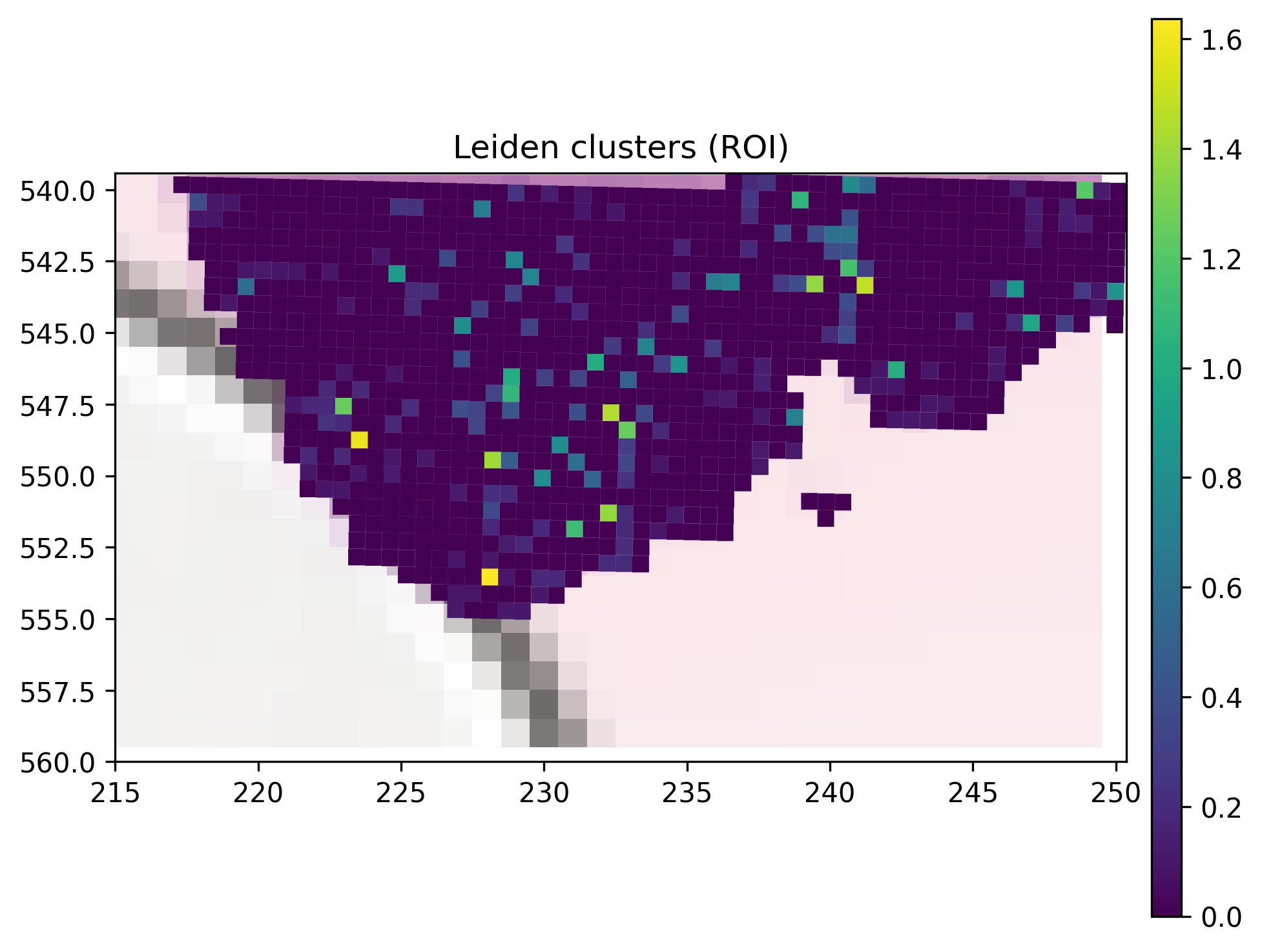
6.4 Zoomed-in region of interest
Use SpatialData’s bounding-box query to zoom into a region of the tissue.
[23]:
# Adjust coordinates to your region of interest
sdata_roi = sdata.query.bounding_box(
    min_coordinate           = [215, 540],
    max_coordinate           = [250, 560],
    axes                     = ('x', 'y'),
    target_coordinate_system = '_downscaled_lowres',
)

sdata_roi.pl.render_images('_lowres_image').pl.render_shapes(
    SHAPE_ELEMENT,
    color      = 'COL18A1:BCL6',
    table_name = 'neighborhood_scores',
    method     = 'matplotlib',
).pl.show(
    coordinate_systems = '_downscaled_lowres',
    title = 'Leiden clusters (ROI)',
)
/home/nr57/.conda/envs/genomics/lib/python3.11/site-packages/spatialdata/_core/_elements.py:105: UserWarning: Key `_square_016um` already exists. Overwriting it in-memory.
  self._check_key(key, self.keys(), self._shared_keys)
/home/nr57/.conda/envs/genomics/lib/python3.11/site-packages/spatialdata/_core/_elements.py:125: UserWarning: Key `neighborhood_scores` already exists. Overwriting it in-memory.
  self._check_key(key, self.keys(), self._shared_keys)
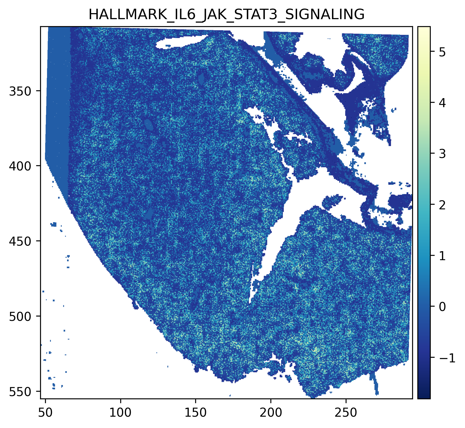
7. Pathway Activity in PC Space
The pcs object returned by downstream_analysis contains spot-level pathway activity scores. We can visualize these spatially to see which biological programs are active in each communication domain.
[24]:
# List the pathway PCs available
print("Available pathway PCs:")
print(pcs.var_names.tolist())
Available pathway PCs:
['HALLMARK_ALLOGRAFT_REJECTION', 'HALLMARK_APOPTOSIS', 'HALLMARK_COAGULATION', 'HALLMARK_COMPLEMENT', 'HALLMARK_EPITHELIAL_MESENCHYMAL_TRANSITION', 'HALLMARK_HYPOXIA', 'HALLMARK_IL2_STAT5_SIGNALING', 'HALLMARK_IL6_JAK_STAT3_SIGNALING', 'HALLMARK_INFLAMMATORY_RESPONSE', 'HALLMARK_INTERFERON_GAMMA_RESPONSE', 'HALLMARK_KRAS_SIGNALING_UP', 'HALLMARK_TNFA_SIGNALING_VIA_NFKB', 'KEGG_APOPTOSIS', 'KEGG_CHEMOKINE_SIGNALING_PATHWAY', 'KEGG_CYTOKINE_CYTOKINE_RECEPTOR_INTERACTION', 'KEGG_FOCAL_ADHESION', 'KEGG_JAK_STAT_SIGNALING_PATHWAY', 'KEGG_MAPK_SIGNALING_PATHWAY', 'KEGG_NOD_LIKE_RECEPTOR_SIGNALING_PATHWAY', 'KEGG_PATHWAYS_IN_CANCER', 'KEGG_TGF_BETA_SIGNALING_PATHWAY', 'KEGG_TOLL_LIKE_RECEPTOR_SIGNALING_PATHWAY', 'WP_ADIPOGENESIS', 'WP_ALLOGRAFT_REJECTION', 'WP_APOPTOSIS', 'WP_BURN_WOUND_HEALING', 'WP_CHEMOKINE_SIGNALING_PATHWAY', 'WP_CIRCADIAN_RHYTHM_GENES', 'WP_DNA_DAMAGE_RESPONSE_ONLY_ATM_DEPENDENT', 'WP_EGFR_TYROSINE_KINASE_INHIBITOR_RESISTANCE', 'WP_EPITHELIAL_TO_MESENCHYMAL_TRANSITION_IN_COLORECTAL_CANCER', 'WP_FOCAL_ADHESION', 'WP_FOCAL_ADHESION_PI3KAKTMTORSIGNALING_PATHWAY', 'WP_FOLATE_METABOLISM', 'WP_HEPATITIS_B_INFECTION', 'WP_IL18_SIGNALING_PATHWAY', 'WP_LUNG_FIBROSIS', 'WP_MALIGNANT_PLEURAL_MESOTHELIOMA', 'WP_MAPK_SIGNALING_PATHWAY', 'WP_NETWORK_MAP_OF_SARSCOV2_SIGNALING_PATHWAY', 'WP_NEUROINFLAMMATION_AND_GLUTAMATERGIC_SIGNALING', 'WP_NUCLEAR_RECEPTORS_METAPATHWAY', 'WP_OREXIN_RECEPTOR_PATHWAY', 'WP_OVERVIEW_OF_PROINFLAMMATORY_AND_PROFIBROTIC_MEDIATORS', 'WP_PHOTODYNAMIC_THERAPYINDUCED_AP1_SURVIVAL_SIGNALING', 'WP_PI3KAKT_SIGNALING_PATHWAY', 'WP_SARSCOV2_INNATE_IMMUNITY_EVASION_AND_CELLSPECIFIC_IMMUNE_RESPONSE', 'WP_SPINAL_CORD_INJURY', 'WP_SUDDEN_INFANT_DEATH_SYNDROME_SIDS_SUSCEPTIBILITY_PATHWAYS', 'WP_TCELL_ACTIVATION_SARSCOV2', 'WP_TGFBETA_RECEPTOR_SIGNALING', 'WP_TGFBETA_RECEPTOR_SIGNALING_IN_SKELETAL_DYSPLASIAS', 'WP_TOLLLIKE_RECEPTOR_SIGNALING_PATHWAY', 'WP_VEGFAVEGFR2_SIGNALING_PATHWAY']
[26]:
# Example: visualize HALLMARK_IL6_JAK_STAT3_SIGNALING
# Replace with a pathway present in your pcs.var_names
pathway_to_plot = 'HALLMARK_IL6_JAK_STAT3_SIGNALING'

if pathway_to_plot in pcs.var_names:
    # Inject pathway activity into the SpatialData table
    sdata.tables['square_016um'].obs[pathway_to_plot] = (
        pcs[:, pathway_to_plot].X.toarray().ravel() if hasattr(pcs.X, 'toarray')
        else pcs[:, pathway_to_plot].X.ravel()
    )
    sdata.tables['square_016um'].obs[pathway_to_plot] = (
        sdata.tables['square_016um'].obs[pathway_to_plot].reindex(
            sdata.tables['square_016um'].obs_names
        ).fillna(0)
    )

    sdata.pl.render_shapes(
        "_square_016um",
        color  = pathway_to_plot,
        method = 'datashader',
        cmap   = 'YlGnBu_r',
    ).pl.show(
        coordinate_systems = '_downscaled_lowres',
        title = pathway_to_plot
    )
else:
    print(f"{pathway_to_plot} not found. Choose from: {pcs.var_names.tolist()}")
/home/nr57/.conda/envs/genomics/lib/python3.11/site-packages/spatialdata_plot/pl/utils.py:1970: UserWarning: Multiple tables contain column 'HALLMARK_IL6_JAK_STAT3_SIGNALING', using table 'pathway_pcs'.
  col_for_color, table_name = _validate_col_for_column_table(
INFO     Using 'datashader' backend with 'sum' as reduction method to speed up plotting. Depending on the reduction
         method, the value range of the plot might change. Set method to 'matplotlib' to disable this behaviour.
/home/nr57/.conda/envs/genomics/lib/python3.11/site-packages/spatialdata/_core/_elements.py:105: UserWarning: Key `_square_016um` already exists. Overwriting it in-memory.
  self._check_key(key, self.keys(), self._shared_keys)
/home/nr57/.conda/envs/genomics/lib/python3.11/site-packages/spatialdata/_core/_elements.py:125: UserWarning: Key `pathway_pcs` already exists. Overwriting it in-memory.
  self._check_key(key, self.keys(), self._shared_keys)
INFO Using the datashader reduction "sum". "max" will give an output very close to the matplotlib result.
8. Differential Expression Across Communication Domains
We perform Wilcoxon rank-sum DE testing across Leiden domains using the raw (unnormalized) gene-expression data.
[29]:
adata_de = neighborhood_scores.copy()

sc.tl.rank_genes_groups(adata_de, groupby='leiden', method='wilcoxon')

sc.pl.rank_genes_groups_heatmap(
    adata_de,
    n_genes          = 10,
    groupby          = 'leiden',
    show_gene_labels = True,
    min_logfoldchange = 0.5,
    dendrogram       = False,
    swap_axes        = True,
    standard_scale   = 'var',
    cmap             = 'viridis',
)
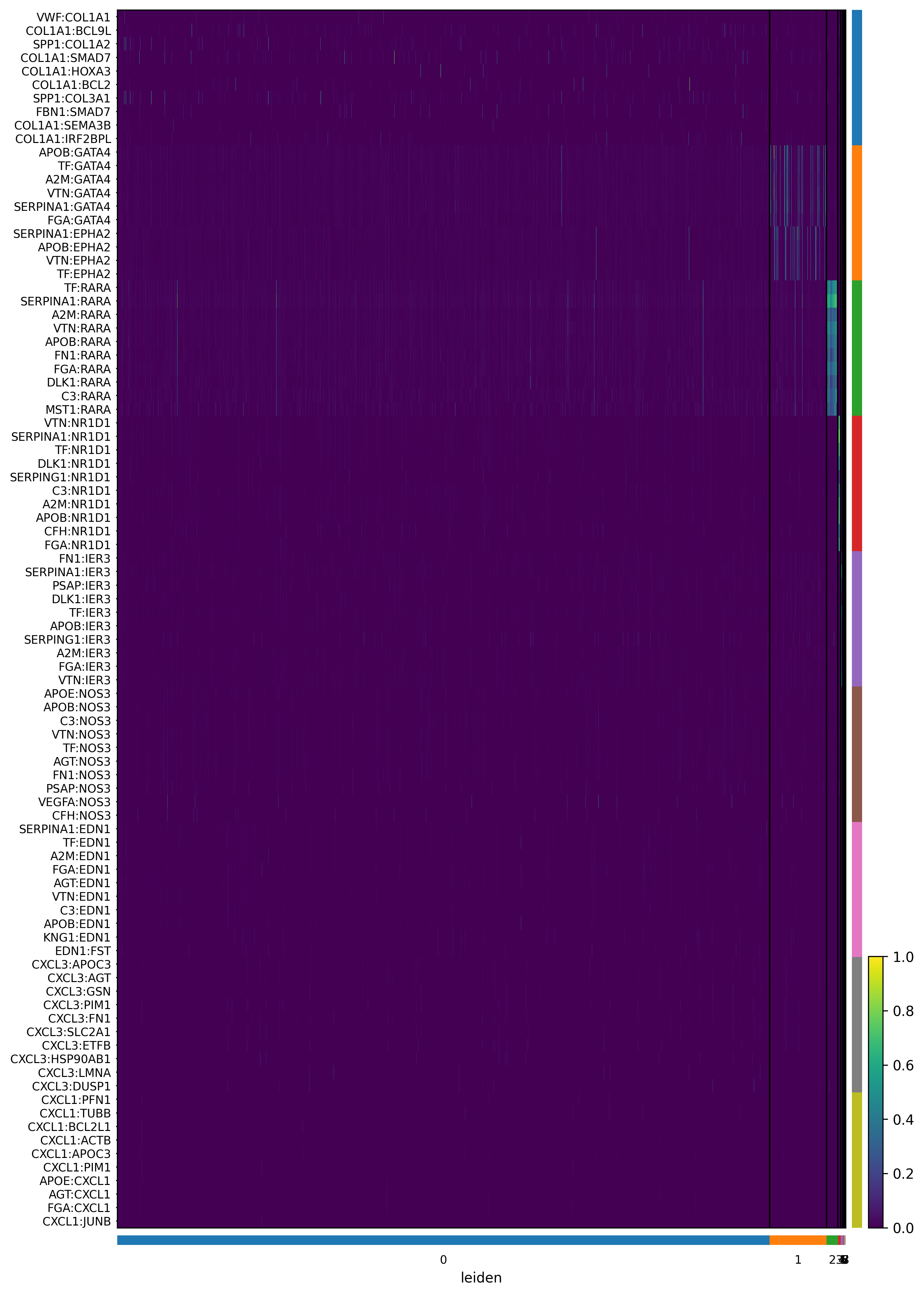
9. Ligand Ranking Analysis
Renoir.ligand_ranking ranks ligands within a selected communication domain by correlating their ligand-target activity scores with known regulatory potential scores. The output is a joint heatmap showing:
y-axis: ligands ranked by their correlation score
x-axis: target genes
Color bars: cell-type origin of ligands (left margin) and targets (top margin)
Inputs required: | Argument | Description | |—|—| | neighbourhood_scores | Renoir output AnnData (with leiden in .obs) | | celltype | Cell-type proportion AnnData (spots × cell types) | | SC | Single-cell reference AnnData (with celltype in .obs) | | ligand_receptor_pairs | DataFrame of known L-R pairs (ligand, receptor columns) | | ligand_target_regulatory_potential | Dict {ligand: {target: score}} | | domain |
Leiden cluster label (string) to analyse |
[32]:
# Load reference files
celltype = sc.read_h5ad(CELLTYPE_PATH)
ligand_receptor_pairs            = pd.read_csv(LR_NATMI_PATH)
ligand_target_regulatory_potential = pkl.load(open(LT_REG_POT_PATH, 'rb'))
SC = sc.read_h5ad(SC_PATH)

# Standardise the cell-type column name in the scRNA reference
if 'cellType' in SC.obs.columns and 'celltype' not in SC.obs.columns:
    SC.obs['celltype'] = SC.obs['cellType']

# Store raw counts for DE testing inside ligand_ranking
neighborhood_scores.raw = neighborhood_scores.copy()

print(f"LR pairs loaded: {ligand_receptor_pairs.shape[0]}")
print(f"Ligands with regulatory potential scores: {len(ligand_target_regulatory_potential)}")
LR pairs loaded: 1804
Ligands with regulatory potential scores: 423
[31]:
# Optional: define custom colours per cell type for the bar annotations
# If not provided, colours are assigned automatically
celltype_colors = {
    'ALB+ APOA2+ Hepatocyte'       : '#A00D0D',
    'FOLR2+ Mac1'                  : '#636458',
    'SPP1+ Mac2'                   : '#A48CF4',
    'CLEC1B+ Endothelial'          : '#6C35DA',
    'LYVE1+ CLEC1B+ Endothelial'   : '#5636A6',
    'PLVAP+ Endothelial'           : '#6C9833',
    'COL3A1 DCN+ Fibroblast'       : '#4E3C2E',
    'POSTN+ Fibroblast'            : '#6E9BF4',
    'KRT19+ Epithelial'            : '#147E50',
    'EPCAM+ Epithelial'            : '#D955DB',
    'GYPA+ BLVRB+ Erythroid'       : '#ACBF18',
    'PF4+ Megakaryocyte'           : '#56CDB4',
    'NKG7+ CD3D+ NKT-cells'        : '#937023',
    'IL7R+ T-cells'                : '#18BFAE',
    'MZB1+ IGLL1+ B-cells'         : '#B5316F',
    'MPO+ PRTN3+ CMP'              : '#92DE84',
    'CPA3+ MAST'                   : '#83B2DD',
    'CLEC10A+ DC2'                 : '#420563',
    'S100A9+ Mono'                 : '#17256A',
    'SPINK2+ SELL+ CLP'            : '#DC82AA',
}
[33]:
# Run ligand ranking for domain '0'
# Change the domain string to any Leiden label of interest
domain_to_analyse = '0'

fig = Renoir.ligand_ranking(
    neighborhood_scores,
    celltype,
    SC,
    ligand_receptor_pairs,
    ligand_target_regulatory_potential,
    domain            = domain_to_analyse,
    receptor_exp      = 0.05,          # min fraction of cells expressing the receptor
    markers           = {'top': 100},  # use top 100 DE genes per cell type as markers
    domain_celltypes  = ['top', 5],   # show top 10 cell types by proportion in the domain
    celltype_colors   = celltype_colors,
)

fig.set_size_inches(28, 14)
#fig.savefig(f'{OUTPUT_DIR}/ligand_ranking_domain{domain_to_analyse}.png', dpi=300, bbox_inches='tight')
fig
[33]: